
Anatomy and Taxonomy of a Fuzzer
Fuzzing is an increasingly popular method for software and hardware quality assurance. A fuzzer is a program or framework that generates pseudo-random inputs, evaluates them, and measures the success or failure of the evaluations. This may be a greatly oversimplified explanation, but it bears the familiar look and feel of test vector sets and unit test frameworks used by engineers since the advent of computers.
For computer scientists and programmers, this article is meant to be a casual introduction to the components, concepts, and construction of fuzz testing systems. For those experienced with the field of fuzzing, this article is meant to isolate features commonly found in fuzzers and relate them to more abstract concepts found in other fields of study. This is not meant to be a canonical representation of the state of the art; there are others who have done an excellent job of both curating and summarizing_1, summarizing_2 detailed publications.
A Fuzzer
In order to establish context for discussing the functionality of complex, modern fuzzing frameworks, let’s first define some minimal parts and/or properties of a fuzzer. The following flow diagram illustrates a minimal fuzzer.
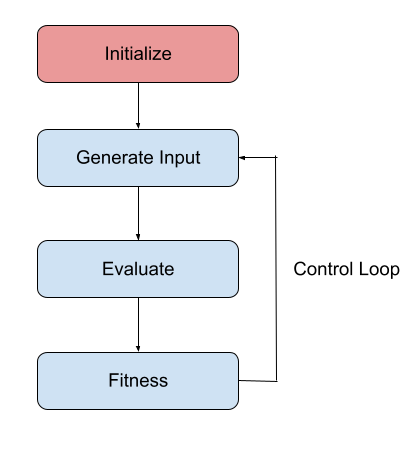
Initialize sets up the environment. This step is optional but typically sets up the evaluation environment, however this can include any number of one time cost activities that would be beneficial to the subsequent effort, such as loading pre-extracted control flow graphs or semantic models of the unit under test.
Generate Input creates a new test case T. Contrary to the simple name and requirement, this step is typically fairly nuanced in practice and has interesting intersections with various fields of mathematics.
Evaluate evaluates T, possibly recording intermediate state information and producing a result, R. This step can be as simple as calling the function to be fuzzed, although in most cases a reset mechanism is required to present each evaluation with a pristine copy of the initialized state. Additionally, intermediate state may be recorded during the evaluation step. Such recordings act as an aid in state space exploration.
Fitness is one or more fitness functions that examine R and determines if T should be reported. The simplest case would be checking R for errant behavior, such as a crash, and reporting T. However, as will be discussed, additional fitness functions can collect data to guide future fuzzing efforts.
Control Loop typically consists of a while(keep_running) type loop, such that the fuzzer repeats the Generate Input, Evaluate, Fitness sequence until the operator is satisfied that the fuzzer has sufficiently explored the state space of the target. The Control Loop might also be used to synchronize work between cores or fuzzing nodes in a distributed setup or run batch tasks to optimize further efforts.
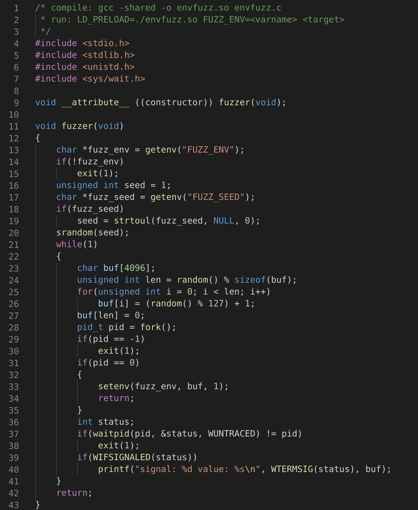
The code above is an updated and simplified version of an inefficient and primitive environment variable fuzzer written by myself over 20 years ago. It would likely find bugs in software today, however there have been many improvements we will get into in later sections that render actually using this pointless. It’s purpose today is to act as a concrete example from which we can identify the anatomical parts of a fuzzer.
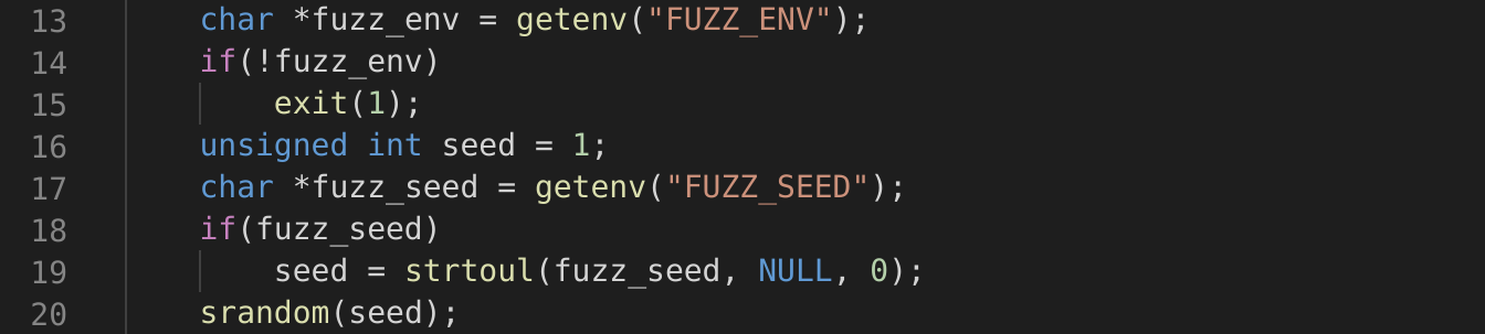
Lines 13-20 correspond to the Initialization step of the fuzzer. This particular fuzzer determines the target environment variable and optionally a seed value to use in the later Generate Input step.

Lines 23-27 correspond to the Generate Input step. Here it generates a pseudo-random ASCII string of a random length up to 4095 bytes or 4096 including the NUL termination.
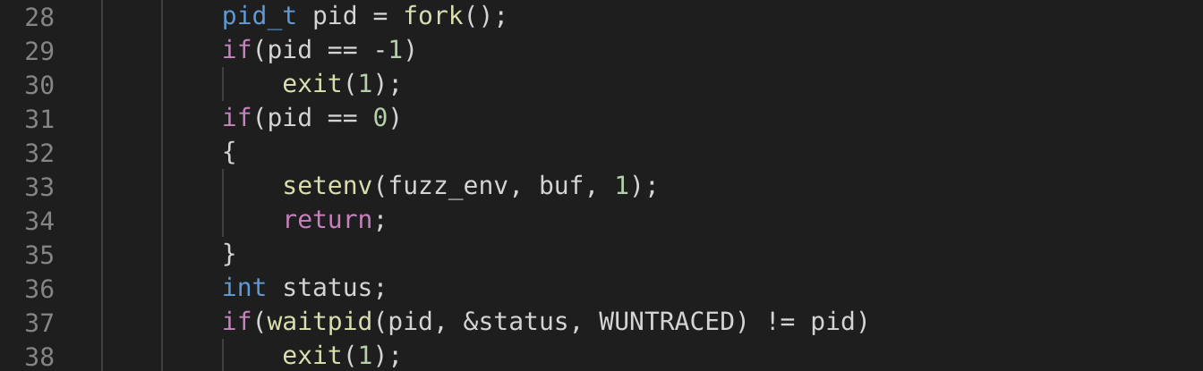
Lines 28-38 correspond to the Evaluate step. Here we see the process use the fork(2) system call which creates an identical child process. The child process can identify itself because fork(2) will return 0 within the child and resume execution. Thus the statement list found in lines 32-35 are only executed by the child. This block sets the target environment variable to the random input generated in the Generate Input step and returns. Return within the execution context of this fuzzer will transfer execution to the entry point of the unit under test, aka the binary we are fuzzing. Line 36 and onward are only executed by the parent process. We can see from line 37-38 it will wait for the child process to exit. Upon resuming the value of status is populated with the exit status of the child process.

Lines 39-40 are our Fitness step. Here we examine the exit status of the child process to determine if it exited due to an unhandled signal. This is ubiquitously known and hated by developers as “a crash”. In the event of a crash, the fuzzer displays the signal number as well as the input that caused the crash.
Finally, we have the Control Loop, this wraps the Generate Input, Evaluate, and Fitness steps.
Input Generation
While the task of input generation can be as simple as generating random values, this section will delve into various input generation optimizations, their benefits, and some areas to expect future optimizations.
The input generation strategy used by most fuzzing frameworks (afl, AFLPlusPLus) relies on maintaining a corpus of inputs, selecting an element from this input corpus, and performing one or more mutations, or alterations to the input. For the sake of this discussion, we will define two new functions, Select and Mutate. Select, as the name implies, selects an element T from some corpus of known inputs, C. Or more simply, T = Select(C). Mutate returns an alteration of T, which we will call T’, or T’ = Mutate(T). Some examples of common mutations are performing single bit flips (xor) within an input, substituting a value within an input, appending new data, or truncating a buffer.
A less common approach used by some fuzzing frameworks (Peach, SPIKE) is use a structured, or grammar based, approach towards input generation. This entails the operator defining the data format and the fuzzer using this definition to generate inputs. This approach has the advantage of being able to handle multi-buffer or multi-part inputs and avoiding the possible pitfall of expending most of the effort exercising initial sanity checks within the unit under test.
Symbolic or constraint solving utilizes a semantic model of the unit under test to solve for values that are advantageous to the operator, such as checksums or magic values (KLEE, bitblaze). In practice this method is often coupled to the Evaluate step, but does not necessarily need to be so. Additionally, some have noted this method as being only applicable in cases where high level source code is available, however modeling the unit under test in the operational semantics of the instruction set it was compiled for is possible.
In recent years advances towards melding these different methods of input generation have been made. For example, if the framework were to derive or infer the type and structure of the input, then the operator would not need to define a grammar in order to reap the benefits of the more targeted mutations of a structured framework. Additionally, constraint solving could simply be used as an expensive (computationally) mutator, possibly of last recourse.
A reader familiar with the subjects of state space exploration or Stochastic optimization might already be noting the similarities found within the field of fuzzing. Optimizations to Select have been done to bias the selection process towards corpus elements with more desirable properties (1, 2).
Mutate has seen many optimizations such as constant mining and substitution, mutator scheduling, and multi-goal effort balancing.
Evaluation
The Evaluate step of the fuzzing process involves executing the generated input while recording desirable metrics. In the following subsections we will discuss the environmental constraints and common ways these are addressed, common methods of instrumenting the unit under test, and the benefits of collecting intermediate metrics throughout the Evaluate step. At minimum, most fuzzers will record faults, signals, and/or exceptions. This is later used in the Fitness step to determine if abnormal or unhandled behavior was experienced as the result of evaluating the input.
Environment
The environment needed for evaluation of test cases typically carries the same execution requirements as the unit under test when built for production, plus the requirement of an immutable state that can be reset. We will refer to this as the Reset Mechanism. It is also important to remove sources of non-determinism from within the unit under test. In most cases these are limited to sources of randomness, such as Address Space Layout Randomization (ASLR) and system random number generators (/dev/urandom for example) but may extend to things such as the current time, process IDs, preemptive scheduling, and external resources such as files, network sockets, and devices. The constraints that the unit under test places upon the Reset Mechanism must be understood in order to create repeatable evaluation results or else the test cases recorded may be meaningless.
End to end fuzzing is generally not feasible given the size and complexity of the exploration space of most software and hardware. A common solution to this is to isolate functionality and use different fuzzers to test components independently. As with unit testing, design of the product components can make this task easier. If a component can be written as reentrant or that any side effects of repetitively invoking are negligible, a Reset Mechanism may be unnecessary.
The de facto Reset Mechanism in most fuzzing frameworks is a forkserver, which is to say that it uses fork(2). The parent keeps the immutable initialized state of the unit under test, allowing it’s child to execute normally with the provided input. The forkserver loosens the requirement of reentrancy, however fork(2) has higher overhead. Work has been done on Linux to reduce the overhead of fork(2) by incorporating fuzzer specific process snapshot and restore mechanisms (1, 2). This being said, both fork(2) and snapshot based forkservers have the limitation of not being able to restore state external to the process, such as files, shared memory, devices, etc. Some modern operating systems, such as Linux, provide namespaces to isolate some types of external resources and can be used in conjunction with fork(2) to allow state resets on more complex fuzzing targets.
A Reset Mechanism that has gained popularity in recent years is to provide a hypervisor using virtualization API’s. On most Unix platforms, such as Linux, this would be KVM and on Windows HyperV.
The advantages of using virtualization are that the restoration overhead is typically much lower than that of traditional forkservers, process external state can be restored, and kernels and binaries can be fuzzed. An interesting project currently under development is FuzzOS. This project not only has a fuzzing optimized host operating system but a fuzzing optimized guest operating system.
If the planned execution environment is an emulator, the Reset Mechanism used will be dependent on how the emulator is constructed. An ideal case would be an emulator that allows in emulator state snapshotting and tracking of modified state, such as dirty memory pages. Unfortunately most emulators are written for the sole purpose of normal execution and are not as efficient as they could be when modified to facilitate a fuzzer’s Reset Mechanism.
Intermediate Metrics
Some examples of types of instrumentation that a fuzzer may perform include recording branching, specific API calls, resource allocation, and type information within the unit under test. These measurements are often approximated to save Evaluate and Fitness execution time in order to process a higher number of inputs, thus optimizing for potential results.
Recording branching allows the fuzzing framework to treat the execution path of the program as an approximation of the state space explored by the test case. At least to this author’s recollection, this was first done in AFL and was probably the first major step towards formalizing automated state space exploration within the field of fuzzing. AFL instruments branch targets, assigning each a unique ID. When the branch target is called a hash, H, is computed from the last branch target ID and the current branch target ID, or H = hash(last, current). This is effectively a unique ID for the edge formed by the nodes last and current within the control flow graph of the unit under test. Then it uses this hash to increment the hash corresponding index within a counting bloom filter, or counting_bloom[H]++. Finally it overwrites the last branch target ID with the current one, thus allowing the next branch target to compute the new edge correctly. Once Evaluate is complete, AFL transforms the counting bloom filter into a bitwise bloom filter where H is used as a byte index and the count at position H in the counting bloom filter is converted to it’s log2 integral equivalent and limited to 128. This compromise allows for the AFL to account for looping within the execution path without the explosive size of accounting for every unique count. Thus the final approximation of the state space traversal of Evaluate is represented using a convenient fixed size surrogate.
Recording specific API calls can allow the fuzzer to identify specific errant behavior, such as command injection, or identify potential sources of user defined input within the unit under test.
Resource utilization can also be recorded at different intervals of execution. This is useful if one of the goals of fuzzing the unit under test is to look for high or exhaustive resource utilization. An example that borrows from the approximation method for control flow graph edge visitation found in AFL would be to have some state hash S and to hook within the unit under test allocations and deallocations. Upon hitting either of these hooks, S is updated to reflect a new state approximation and it’s value recorded into the counting bloom filter. A more elaborate example targeting Java can be found in HotFuzz.
Instrumentation
With additional instrumentation, the fuzzer can collect other useful information about the intermediate states of execution. The most common methods of inserting instrumentation into the unit under test we will discuss are as follows:
- Compiler pass(es)
- Dynamic Binary Instrumentation (DBI)
- Interpreter or runtime modifications
- Emulator facilitated
- Runtime linker interfaces
- CPU mechanisms
Depending on the type of instrumentation, a fuzzer may choose to use one type of instrumentation over another. It is often the case that a fuzzer uses multiple types of instrumentation.
Inserting instrumentation via the compiler requires adding an additional pass to the compilation process. In modern modular compilers this can be done during the command line invocation of the compiler and many of the major fuzzing frameworks provide such modules. The compiler also has access to the higher level semantics of the unit under test. Depending on the features of the fuzzing framework, these high level semantics can prove useful in state space exploration. Instrumentation via the compiler does have the requirement that the operator of the fuzzer has source code to the unit under test.
As a side note, modern compilers can optionally provide memory sanity checking at runtime. For the developers reading, this would be runtime checks like StackGuard, AddressSanitizer, or guard pages. Inclusion of such checks by a fuzzer allows it to identify exactly the point an invalid read or write to memory occurred. This is important because not all behavior violations trigger other observable behavior such as crashes. Additionally this prevents the unit under test from executing past the point of violating these invariants, which typically leads to higher manual deduplication workload for the fuzzer operator. It should also be noted that different efforts have been to insert such checks to existing compiled binaries and/or bytecode with limited and varying success.
When source code is not available a common alternative for inserting instrumentation is to use a DBI framework such as Intel PIN, DynamoRIO, or DynInst. The DBI allows rewriting and insertion of instructions either to a binary on disk or to a binary as it executes. This removes the requirement for source, however the fuzzer operator still is required to have a platform capable of executing the binary in the first place.
If the unit under test is written in a language that requires an interpreter, a logical place for inserting instrumentation might be the interpreter itself. How this is done is highly dependent on the interpreter, how it is implemented and what features are provided by the interpreter. When the environment of the unit under test provides reflection and code rewriting, a fuzzer can be implemented by hooking or replacing the code/bytecode loading mechanism. When a new code or bytecode is loaded, the fuzzing framework rewrites it to include the necessary instrumentation. When such a mechanism is unavailable, it may be necessary to patch the runtime itself.
Instrumentation within an emulated environment depends heavily on how the emulator is implemented. The simplest but probably most universal way is to rewrite the unit under test prior to execution in the same manner as a DBI. This however has the side effect that the changes may be observable to the unit under test, as with a DBI. If the emulator utilizes a Just In Time, or JIT, compilation system, instrumentation can be inserted during or just prior to lowering the higher level instruction sequences to native instructions. When the emulator doesn’t use a JIT instrumentation can still be inserted by modification of instruction behavior. Often this is the case whether a JIT is employed or not when doing symbolic fuzzing on closed source targets as the instruction stream is modeled then evaluated or solved for instead of just directly executed.
The runtime linker can also be used to insert instrumentation relevant to fuzzing. The fuzzer may abuse library link and load order in order to insert itself and it’s hooks into a process. How this is done is highly dependent on the constraints specified by the binary format itself. The simple environment variable fuzzer discussed previously in this article utilizes LD_PRELOAD in order to insert its forkserver into the process of the unit under test. Additionally a fuzzer can use the runtime linker to hook shared library functions utilized by the unit under test. We will discuss the ramifications of this in the next section.
Modifications to the operating system can also be used as an instrumentation mechanism. In the case of most modular operating systems, this can be done via a kernel module. When this is not an option, the operating system can be modified directly either via source or runtime patching. Kernel based instrumentation methods typically provide a feedback mechanism such that the kernel notifies and/or collects information about the unit under test during evaluation and passes it to the fuzzing process. This can be especially useful in the case of resource consumption monitoring, as most operating systems have such mechanisms in them already for the purposes of profiling applications. Another example of note would be to alter the behavior of kernel interfaces such that modifications to process external resources such as files are able to be reset efficiently.
Many CPUs contain mechanisms that can either be used to instrument or to collect metrics analogous to ones that fuzzers typically instrument for. The simplest case would be inserting breakpoints into the unit under test and that the fuzzing framework would provide a breakpoint handler to record or alter the normal behavior. On x86 CPUs the Trap Flag can be set to trigger invocation of the breakpoint handler on execution of every instruction. The disadvantage is that breakpoints require multiple CPU context switches to process and thus execution time is wasted. Many modern general purpose CPUs performance profiling features that cause the CPU to record or trap when a branch instruction is executed. This is often architecture or even vendor specific (1, 2) and may require additional post processing. The overhead and limitations are highly implementation specific, however a few fuzzing frameworks make use of such features (1, 2).
Fitness Function(s)
Fitness functions are used within the fuzzer to determine whether the evaluation expressed any behavior worth saving. In the most basic case, this would be that Evaluate resulted in an observable defect, such as a crash, assertion, or an unhandled exception. Modern fuzzing frameworks typically have additional fitness functions to examine the intermediate metrics recorded during the evaluation. These tests typically identify behavior that has not yet been observed by the fuzzer and save a copy to the template corpus used by Select.
For example, in the previous section we discussed the fixed sized execution path surrogate that AFL computes during the Evaluate step. In the Fitness step it compares the Evaluate generated value with a global accumulator. This comparison simply needs to identify if a non-zero value exists within the new value where a zero value exists within the accumulator. If such a value exists, the test case is saved to the working corpus used by Select and the generated value is merged (logical OR) into the accumulator. This approximation is both computationally fast, requires a small fixed amount of memory, and is fairly accurate for small paths.
Fitness functions can also identify evaluation results that provide additional user input paths. For example if the fuzzer logs a call to open(2) during evaluation that returns ENOENT, the Fitness function would append this to the working corpus and subsequent iterations of the control loop would try to supply the filename specified in the open(2) call. execve(2) calls that return ENOENT can be examined to determine if the filename argument contains components specified by the test case. Such a mechanism could also be used, and has by the author, to identify command execution vulnerabilities. This can be further filtered by altering the suspected test case components and examining the Evaluate resultant to see if the contents of the filename argument changed as well.
Summary
At the start of this article we listed some of the reasons that people fuzz today and we laid out a framework for discussing the minimal components of a fuzzer. This framework defines an Initialization step as well as a Control Loop that repeatedly iterates over the Generate Input, Evaluate, and Fitness steps. Through discussing how each of the steps can and typically are implemented, we saw how over time fuzzing frameworks and their components have become more robust while finding issues faster. In doing so, we were able to show that many of the improvements come from the understanding of other fields and that likely new ones will as well. Finally, we hope this was a pleasant and informative read.